SEIS

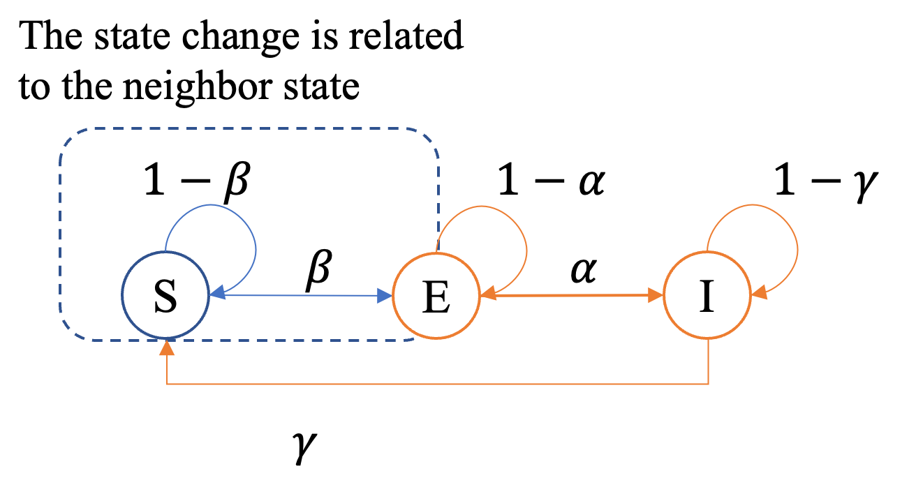
The SEIS Model [1] assumes that infection spreads only through links between neighboring nodes in a graph \(G=(V,E)\). Each node is in one of three states: \(S\) (susceptible), \(E\) (exposed/incubating), or \(I\) (infected). A susceptible node \(i\) becomes exposed by its infected neighbors \(j \in N(i)\) with rate \(\beta\), exposed nodes become infectious with rate \(\alpha\), and infected nodes recover back to susceptible with rate \(\gamma\):

\[\begin{split}\begin{aligned} \frac{dS_i}{dt} &= -\beta \sum_{j\in N(i)} S_i I_j + \gamma I_i, \\ \frac{dE_i}{dt} &= \beta \sum_{j\in N(i)} S_i I_j - \alpha E_i, \\ \frac{dI_i}{dt} &= \alpha E_i - \gamma I_i . \end{aligned}\end{split}\]

Implementation

Node transitions follow three rules:

1. if a \(S\) state node has \(I\) state neighbors, each \(I\) state neighbor exposes the \(S\) state node with probability \(\beta\) (S→E);

2. the \(E\) state node becomes \(I\) with probability \(\alpha\) (E→I);

3. the \(I\) state node is recovered to the \(S\) state with probability \(\gamma\) (I→S).

We represent node states with two Boolean indicator vectors \(h, e \in \{0,1\}^N\):

• \((h_i,e_i)=(0,0)\) denotes Susceptible (S),

• \((h_i,e_i)=(1,1)\) denotes Exposed (E),

• \((h_i,e_i)=(1,0)\) denotes Infected (I).

The update of the system at step \(k\) is decomposed into three stages:

1. Each infected neighbor \(j\) of node \(i\) transmits a log-probability contribution for exposure (S→E)

\[m_{ji}^{(k)} = \mathbf{1}\!\left(h_j^{(k-1)}=1 \land e_j^{(k-1)}=0\right)\,\log(1-\beta)\]

2. Node \(i\) collects contributions from all neighbors \(N(i)\) to compute its exposure probability

\[m_i^{(k)} = 1 - \exp\!\left( \sum_{j \in N(i)} m_{ji}^{(k)} \right)\]

3. The indicator variables are updated with independent uniform random variables \(U_i^{\mathrm{exp}}, U_i^{\mathrm{inf}}, U_i^{\mathrm{rec}} \sim \mathrm{Uniform}(0,1)\)

\[\begin{split}\begin{aligned} h_i^{(k)} &= \begin{cases} 1, & \text{if } (U_i^{\mathrm{exp}} < m_i^{(k)}) \land h_i^{(k-1)}=0 , \\[4pt] 0, & \text{if } (U_i^{\mathrm{rec}} < \gamma) \land (h_i^{(k-1)}=1 \land e_i^{(k-1)}=0), \\[4pt] h_i^{(k-1)}, & \text{otherwise}, \end{cases} \\[6pt] e_i^{(k)} &= \begin{cases} 1, & \text{if } (U_i^{\mathrm{exp}} < m_i^{(k)}) \land h_i^{(k-1)}=0, \\[4pt] 0, & \text{if } (U_i^{\mathrm{inf}} < \alpha) \land e_i^{(k-1)}=1 , \\[4pt] e_i^{(k-1)}, & \text{otherwise}, \end{cases} \\[6pt] \end{aligned}\end{split}\]

Status

During the simulation, a node can be in one of the following states:

Status	Code
Susceptible	0
Infected	1
Exposed	2

SEISModel

class fs_gplib.Epidemics.SEISModel(data, seeds, infection_beta: float, removal_gamma: float, latent_alpha: float, device='cpu', use_weight: bool = False, rand_seed=None)

Bases: DiffusionModel

SEIS (Susceptible-Exposed-Infected-Susceptible) diffusion model on static graphs.

Each node starts as susceptible or infected (seed). At every step each infected neighbor independently exposes a susceptible node with probability \(\beta\) (S→E), exposed nodes become infectious with probability \(\alpha\) (E→I), and infected nodes recover back to susceptible with probability \(\gamma\) (I→S).

Returned node states are encoded as: 0 = susceptible, 1 = infected, 2 = exposed.

Parameters:

• data (torch_geometric.data.Data) -- PyTorch Geometric Data object representing graph \(G=(V,E)\). Must contain edge_index (the edge set \(E\)) and num_nodes (\(|V|\)). When use_weight is True, edge_attr supplies per-edge weights \(w_{ji}\).

• seeds (list[int] | float) -- Nodes whose initial state is Infected. Pass a list of node IDs, or a float in (0, 1) to infect that fraction of nodes chosen uniformly at random.

• infection_beta (float) -- Per-contact exposure probability \(\beta \in [0,1]\) (S→E).

• removal_gamma (float) -- Per-step recovery probability \(\gamma \in [0,1]\) (I→S).

• latent_alpha (float) -- Per-step incubation/progression probability \(\alpha \in [0,1]\) (E→I).

• device (str | int) -- (optional) 'cpu' or a CUDA device index. Defaults to 'cpu'.

• use_weight (bool) -- (optional) If True, each edge \((j,i)\) carries a weight \(w_{ji}\) from data.edge_attr and the exposure probability becomes \(\beta w_{ji}\). If False all weights default to 1 (i.e. \(w_{ji}=1\)). Defaults to False.

• rand_seed (int | None) -- (optional) Random seed used when seeds is a float. Defaults to None.

run_iteration()

Execute a single simulation step.

The internal node_status is updated so that subsequent calls continue from the latest state.

Returns:

Node states after one step, shape (1, N).

Return type:

torch.Tensor

run_iterations(times)

Execute times simulation steps sequentially.

The internal node_status is updated in-place so that subsequent calls continue from the latest state.

Parameters:

times (int) -- Number of steps to run.

Returns:

Node states at final step, shape (1, N).

Return type:

torch.Tensor

run_epoch(iterations_times)

Run a single Monte-Carlo epoch (one independent realisation).

Node states are re-initialised before the epoch starts.

Parameters:

iterations_times (int) -- Number of simulation steps per epoch.

Returns:

Node states at final step of the epoch, shape (1, N).

Return type:

torch.Tensor

run_epochs(epochs, iterations_times, batch_size=200)

Run multiple independent Monte-Carlo epochs in batches.

Node states are re-initialised before the run.

Parameters:

• epochs (int) -- Total number of independent realisations.

• iterations_times (int) -- Number of simulation steps per epoch.

• batch_size (int) -- (optional) Number of epochs processed in parallel per batch. Defaults to 200.

Returns:

Node states at final step of all epochs, shape (epochs, N).

Return type:

torch.Tensor

References

[1]

Fan M, Li M Y, Wang K. Global stability of an SEIS epidemic model with recruitment and a varying total population size[J]. Mathematical biosciences, 2001, 170(2): 199-208.